Excel 4 Teachers pt.1 – from UMS to grades

How amazing would it be if you could be that colleague with the colour-coded Excel spreadsheet which calculates totals, tells you the UMS points AND transfers this into grades all in the time it takes to slap three kids into detention for sticking their bogies to the door handle? Well now you can, and here’s how…

Step 1: set up your columns

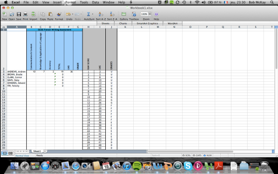
I’ve set my sheet up for Unit 4 of the Edexcel GCSE in French, but you can obviously do this for any assessment, scheme and exam board. First of all, simply head your columns appropriately for your marks:

My spreadsheet is set up with columns for students’ names and their marks.

The columns and rows are named by Excel with numbers and letters: column A contains the names, columns B, C and D the marks and columns E, F and G the total, UMS and grade respectively. Thus, cell G3 will contain Andrew’s grade for the task.

Step 2: totalling up the marks

Stop being that teacher sat at their desk with a calculator your HoD ordered from the supply catalogue – get Excel to do it for you. In the total column, type the following formula:

=SUM(B3:D3)

Then press enter. This means that all of the cells between (and including) B3 and D3 will be totalled together in the column containing the formula. You can then copy and paste this into all of the cells beneath (CTRL+C to copy, CTRL+V to paste). Now, when you type numbers into the first three columns of your sheet, Excel will total them up for you. Bear in mind that the total will (logically) show as zero until you input some data. Try putting a ‘1’ into each column and checking that the total comes out as three.

Watch out! – B3:D3 is the range of columns I’m totalling in this spreadsheet, but it may not be in yours – check which columns you actually want to total and adapt the formula accordingly.

Step 3: calculate the UMS

Now, instead of looking up each individual student’s UMS score, you can programme Excel to do it for you.

To do this, you first need to find the raw score to UMS conversion table for your exam board, (the Edexcel 2011 French conversion table can be found here). I have then just copied and pasted the table for GCSE writing into the empty columns on my spreadsheet:

My spreadsheet now contains the exam board’s raw score to UMS conversion data.

Beware! The raw scores and UMS must be entered in ascending order for this to work (ie: starting at 1 and working upwards numerically as you go down the sheet).

What you now need the spreadsheet to do is look up the total number of points your student was awarded (cell E3) and then look up the corresponding number of UMS points and put this figure into column F. Unsurprisingly the formula for this is ‘LOOKUP’:

=LOOKUP(E3, H3:H62, I3:I62)

This formula means the the spreadsheet will look up the value in cell E3, find it somewhere between cells H3 and H62 and then display the value in the next column (cells I3 to I62). Thus, if Andrew is awarded marks of 10, 7 and 2, with a total of 19, the spreadsheet looks this value up and calculates the relevant UMS points as 36.

Unfortunately you can’t just copy and paste this formula into the cells beneath, beacuase it will change the search ‘vectors’ (ie: the range of cells where your raw marks and UMS are stored). To stop it from doing this, simply highlight the two search vectors as shown and press F4:

 

Watch out! If you’re using a Mac (like me!) you’ll need to type the $ signs in manually, but on a PC pressing F4 will do that for you. Your formula is now ready to copy and paste into all the cells beneath.

Step 4: calculate the grades

Our final step is to have the spreadsheet convert the numerical UMS into letter grades. To do this, we first need to enter the grades next to their corresponding UMS according to the exam board’s grade boundaries, which can usually be found in the course specification:

Now all we need to do is repeat the same process for step 2, but modifying the formula so that it searches columns I and J instead of H and I:

=LOOKUP(F3*2, $I$3:$I$62, $J$3:$J$62)

Note that I have also inserted *2 next to F3; this is because for the Edexcel French GCSE, students submit two pieces of controlled writing, but we only have the marks for one. I therefore need to double the UMS score as the exam board’s grade boundaries are based on the premise that the UMS are totalled for two pieces of work.

Once copied and pasted, this gives us a filled-out spreadsheet with each students’ grade:

Hopefully none of that was too complicated. I’m certainly no genius when it comes to computers, so if I can do it anyone can! If you get stuck, comment below and I’ll see if I can help!